Weighted graphs

K08 Δομές Δεδομένων και Τεχνικές Προγραμματισμού

Κώστας Χατζηκοκολάκης

Weighted graphs

• Graphs with numbers, called weights, attached to each edge
  • Often restricted to non-negative
• Directed or undirected
• Examples
  • Distance between cities
  • Cost of flight between airports
  • Time to send a message between routers

Weighted graphs

• Adjacency matrix representation $$T[i,j] = \begin{cases} w_{i,j} & \text{if } i,j\text{ are connected} \\ \infty & \text{if } i\neq j\text{ are not connected} \\ 0 & \text{if } i = j \end{cases} $$
• Similarly for adjacency lists

Example weighted graph

Example weighted graph

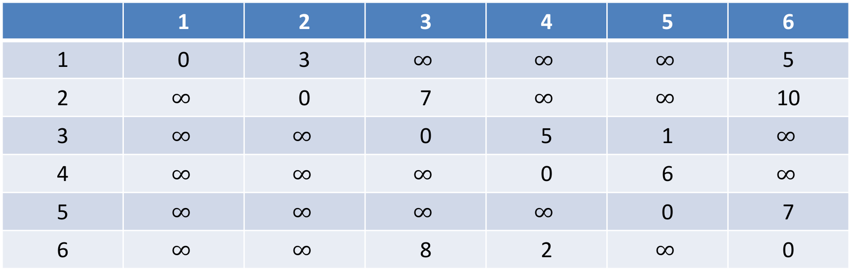
Adjacency matrix

Shortest paths

• The length of a path is the sum of the weights of its edges
• Very common problem
  • find the shortest path from $s$ to $d$
• Examples
  • Shortest route between cities
  • Cheapest connecting flight
  • Fastest network route
  • …

Shortest path from vertex 1 to vertex 5

Shortest path problem

Two main variants:

• Single source $s$
  • Find the shortest path from $s$ to each node
  • Dijkstra's algorithm
    • Only for non-negative weights (important!)
• All-pairs
  • Find the shortest path between all pairs $s,d$
  • Floyd-Warshall algorithm
    • Any weights

Dijkstra's algorithm

Main ideas:

• Keep a set $W$ of visited nodes
  • Start with $W = \{s\}$ $\quad$ (or $W = \{\}$)
• Keep a matrix $\Delta[u]$
  • Minimum distance from $s$ to $u$ passing only through $W$
  • Start with $\Delta[u] = T[s,u]$ $\quad$(or $\Delta[s] = 0, \Delta[u] = \infty$)
• At each step we enlarge $W$ by adding a new vertex $w \not\in W$
  • $w$ is the one with minumum $\Delta[w]$

Dijkstra's algorithm

Main ideas:

• Adding $w$ to $W$ might affect $\Delta[u]$
  • For some neighbour $u$ of $w$
• We might now have a shorter path to $u$ passing through $w$
  • Of the form $s \to\ldots\to w \to u$
  • If $\Delta[u] > \Delta[w] + T[w,u]$
• In this case we update $\Delta$
  • $\Delta[u] = \Delta[w] + T[w,u]$

Example graph

Expanding the vertex set w in stages

Expanding the vertex set w in stages

Expanding the vertex set w in stages

Expanding the vertex set w in stages

Expanding the vertex set w in stages

Expanding the vertex set w in stages

Expanding the vertex set w in stages

Expanding the vertex set w in stages

Expanding the vertex set w in stages

Expanding the vertex set w in stages

Expanding the vertex set w in stages

Dijkstra's algorithm in pseudocode

// Δεδομένα
src  : αρχικός κόμβος
dest : τελικός κόμβος

// Πληροφορίες που κρατάμε για κάθε κόμβο v
W[u]     : 1 αν ο u είναι στο σύνολο W, 0 διαφορετικά
dist[u]  : ο πίνακας Δ
prev[u]  : ο προηγούμενος του v στο βέλτιστο μονοπάτι

// Αρχικοποίηση: W={} (εναλλακτικά μπορούμε και W={src})
for each vertex u in Graph  
  dist[u] = INT_MAX    // infinity
  prev[u] = NULL
  W[u] = 0

dist[src] = 0

Dijkstra's algorithm in pseudocode

// Κυρίως αλγόριθμος
while true  
    w = vertex with minimum dist[w], among those with W[w] = 0

    W[w] = 1
    if w == dest
        stop
        // optimal cost = dist[dest]
        // optimal path = dest <- prev[dest] <- ... <- src (inverse)

    for each neighbor u of w
        if W[u] == 1
            continue
        alt = dist[w] + weight(w,u)     // κόστος του src -> ... -> w -> u
        if alt < dist[u]                // καλύτερο από πριν, update
            dist[u] = alt
            prev[u] = w

Using a priority queue

• Finding the $w\not\in W$ with minumum $\Delta[w]$ is slow
  • $O(n)$ time
• But we can use a priority queue for this!
  • We only keep vertices $w\not\in W$ in the queue
  • They are compared based on their $\Delta[w]$
    (each $w$ has “priority” $\Delta[w]$)
• Careful when $\Delta[w]$ is modified!
  • Either use a priority queue that allows updates
  • Or insert multiple copies of each $w$ with different priorities
    • the queue might contain already visited vertices: ignore them

Dijkstra's algorithm with priority queue

// Δεδομένα
src  : αρχικός κόμβος
dest : τελικός κόμβος

// Πληροφορίες που κρατάμε για κάθε κόμβο u
W[u]     : 1 αν ο v είναι στο σύνολο W, 0 διαφορετικά
dist[u]  : ο πίνακας Δ
prev[u]  : ο προηγούμενος του v στο βέλτιστο μονοπάτι
pq       : Priority queue, εισάγουμε tuples {u,dist[u]}
           συγκρίνονται με βάση το dist[u]

// Αρχικοποίηση: W={} (εναλλακτικά μπορούμε και W={src})
prev[src] = NULL
dist[src] = 0
pqueue_insert(pq, {src,0})  // dist[src] = 0

Dijkstra's algorithm with priority queue

// Κυρίως αλγόριθμος
while pq is not empty
    w = pqueue_max(pq)  // w with minimal dist[u]
    pqueue_remove_max(pq)

    if exists(W[w])     // το w μπορεί να υπάρχει πολλές φορές στην ουρά (αν
        continue        // δεν κάνουμε replace), και να είναι ήδη visited
    W[w] = 1
    if w == dest
        stop            // optimal cost/path same as before

    for each neighbor u of w
        if exists(W[u])
            continue
        alt = dist[w] + weight(w,u)     // cost of src->...->w->u
        if !exists(dist[u]) OR alt < dist[u]
            dist[u] = alt
            prev[u] = w
            pqueue_insert(pq, {u,alt})  // προαιρετικά: replace αν υπάρχει ήδη!

stop // pq άδειασε πριν βρούμε το dest => δεν υπάρχει μονοπάτι

Notation

• $s\to d$
  • Direct step step from $s$ to $d$
• $s \xrightarrow{W} d$
  • Multiple steps $s \to \ldots \to d$
  • All intermediate steps belong to the set $W\subseteq V$
• $s \xRightarrow{W} d$
  • Shortest path among all $s \xrightarrow{W} d$
  • So $s \xRightarrow{V} d$ is the overall shortest one

Proof of correctness

• We need to prove that $\Delta[u]$ is the minimum distance to $u$
  • after the algorithm finishes
• But it's much easier to reason step by step
  • we need a property that holds at every step
  • this is called an invariant (property that never changes)

Proof of correctness

Invariant of Dijkstra's algorithm

• $\Delta[u]$ is the cost of the shortest path passing only through $W$
• And the shortest overall when $u\in W$

Formally:

1. For all $u\in V\;$ the path $s\xRightarrow{W} u$ has cost $\Delta[u]$

2. For all $u \in W$ the path $s\xRightarrow{V} u$ has cost $\Delta[u]$

Proof: induction on the size of $W$, for both (1), (2) together

Proof of correctness

Base case $W = \{ s\}$

• Trivial, the only path $s \xrightarrow{W} u$ is the direct one $s\to u$
• For (1): its cost is exactly $T[s,u] = \Delta[u]$
  • initial value of $\Delta[u]$
• For (2): the only $u\in W$ is $s$ itself

Proof of correctness

Inductive case

• Assume $|W|=k$ and (1),(2) hold
• The algorithm
  • Updates $W$, adding a new vertex $w\not\in W$
  • Updates $\Delta[u]$ for all neighbours $u$ of $w$
• Let $W’,\Delta'$ be the values after the update
• Show that (1),(2) still hold for $W’,\Delta'$

Proof of correctness

We start showing that (2) still holds for $W’,\Delta'$

• The interesting vertex is the $w$ we just added
  • Vertices $u \neq w$ are trivial from the induction hypothesis
• Show: $s\xRightarrow{V} w$ has cost $\Delta’[w]$
  • Note: $\Delta’[w] = \Delta[w]$ (we do not update $\Delta[w]$)
  • We already know that $s\xRightarrow{W} w$ has cost $\Delta[w]$ (ind. hyp)
  • So we just need to prove that there is no better path outside $W$

Proof of correctness

• Assuming such path exists, let $r$ be its first vertex outside $W$
  • So the path $s \xRightarrow{W} r \xRightarrow{V} w$ has cost $c < \Delta[w]$
  • So the path $s \xRightarrow{W} r$ has cost at most $c < \Delta[w]$ (no negative weights!)
  • So $\Delta[r] < \Delta[w]$
• Impossible! We chose $w$ to be the one with min $\Delta[w]$

Proof of correctness

It remains to show (1) for $W’,\Delta'$

• Take some arbitrary $u$
  • Let $c$ be the cost of $s \xRightarrow{W’} u$
  • Show: $c=\Delta’[u]$
• Three cases for the optimal path $s \xRightarrow{W’} u$
• Case 1: the path does not pass through $w$
  • So it is of the form $s \xRightarrow{W} u$
  • This path has cost $\Delta[u]$ (induction hypothesis)
  • No update: $\Delta’[u] = \Delta[u] = c$

Proof of correctness

• Case 2: $w$ is right before $u$
  • So the path is of the form $s \xRightarrow{W} w \to u$
  • The cost of $s \xRightarrow{W} w$ is $\Delta[w]$ (induction hypothesis)
  • So $c = \Delta[w] + T[w,u]$
  • So the algorithm will set $\Delta’[u] = \Delta[w] + T[w,u]$
    when updating the neighbours of $w$
  • So $c = \Delta’[u]$

Proof of correctness

• Case 3: some other $x$ appears after $w$ in the path
  • So the path is of the form $s \xRightarrow{W} w \to x \xRightarrow{W} u$
  • But the path $s \xRightarrow{W} w \to x$ is no shorter than $s \xRightarrow{W} x$
    • From the induction hypothesis for $x \in W$
  • So $s \xRightarrow{W} x \to u$ is also optimal, reducing to case 1!

Complexity

Without a priority queue:

• Initialization stage: loop over vectices: $O(n)$
• The while-loop adds one vertex every time: $n$ iterations
• Finding the new vertex loops over vertices: $O(n)$
  • same for updating the neighbours
• So total $O(n^2)$ time

Complexity

With a priority queue:

• Initialization stage: loop over vectices, so $O(n)$
• Count the number of updates (steps in the inner loop)
  • Once for every neighbour of every node: $e$ total
  • Each update is $O(\log n)$ (at most $n$ elements in the queue)
• Total $O(e\log n)$
  • Assuming a connected graph ($e \ge n$)
  • And an implementation using adjacency lists
• Only good for sparse graphs!
  • But $O(n\log n)$ can be hugely better than $O(n^2)$

The all-pairs shortest path problem

• Find the shortest path between all pairs $s,d$
• Floyd-Warshall algorithm
• Any weights
  • Even negative
  • But no negative loops (why?)

The all-pairs shortest path problem

Main idea

• At each step we compute the shortest path through a subset of vertices
  • Similarly to $W$ in Dijkstra
  • But now the set at step $k$ is $W_k = \{ 1,\ldots, k\}$
    • Vectices are numbered in any order
• Step $k$: the cost of $i \xRightarrow{W_k} j$ is $A_k[i,j]$
  • Similar to $\Delta$ in Dijstra (but for all pairs $i,j$ of nodes)

Floyd-Warshall algorithm

• The algorithm at each step computes $A_k$ from $A_{k-1}$
• Initial step $k=0$
  • Start with $A_0[i,j] = T[i,j]$
  • Only direct paths are allowed

Floyd-Warshall algorithm

$k$-th iteration: the optimal $i \xRightarrow{W_k} j$ either passes thorugh $k$ or not. $$ A_k[i,j] = \min \begin{cases} A_{k-1}[i,j] \\ A_{k-1}[i,k] + A_{k-1}[k,j] \end{cases} $$

Floyd-Warshall algorithm in pseudocode

void floyd_warshall() {

    for (int i = 0; i <= size-1; i++)
        for (int j = 0; j <= size-1; j++)
            A[i][j] = weight(i, j)

    for (int i = 0; i <= size-1; i++)
        A[i][i] = 0;

    for (int k = 0; k <= size-1; k++)
        // Compute A_k from A_{k-1}
        for (int i = 0; i <= size-1; i++)
            for (int j = 0; j <= size-1; j++)
                if (A[i][k] + A[k][j] < A[i][j])
                    A[i][j] = A[i][k] + A[k][j]
}

A is the current $A_k$ at every step $k$.

Complexity

• Three simple loops of $n$ steps
• So $O(n^3)$
• Not better than $n$ executions of Dijkstra in complexity
  • But much simpler
  • Often faster in practice
  • And works for negative weights

Readings

• T. A. Standish. Data Structures , Algorithms and Software Principles in C. Chapter 10

• A. V. Aho, J. E. Hopcroft and J. D. Ullman. Data Structures and Algorithms. Chapters 6 and 7